I like to think I’m principled in my approach to life. I don’t play the lottery. I buy the cheapest apartment insurance possible. I’ve run the numbers.

So why the hell do I vote?

By a back-of-the-envelope estimate, future me will waste about ten hours of my life voting in federal elections. Ten hours for something I’m pretty sure is useless. This is deeply unsettling, so naturally, I sat down and spent far more than ten hours proving whether those ten hours were, in fact, going to be wasted.

The calculation

The question we’re trying to answer is: what are the chances your vote actually matters? And I don’t mean “matters” in the warm-fuzzy-civic-participation sense that teachers tell you about in high school. I mean: what is the probability that your individual vote literally changes who becomes president?

This breaks down into two sub-questions:

1. What’s the probability your vote flips your state?
2. Given your vote flipped your state, what is the probability that flipping your state flips the whole election?

Multiply these together and you get the probability your vote changes the outcome. Then multiply THAT by how much better you think your candidate is than the other candidate, and you get a dollar amount representing the expected value of voting.

Mathematically:

A quick note on that \(\Delta V\) term: we use altruistic value – how much better society would be with your candidate – rather than personal gain. Why?

Because even if a candidate promised you $1 million personally if they win, the probability terms we are about to calculate are so small that your expected value would round to $0. Voting for pure self-interest makes no sense. The only coherent consequentialist framework for voting is caring about total societal value.

So that’s what we’ll estimate.

Part 1: What are the chances your vote flips the election?

Understanding polling error

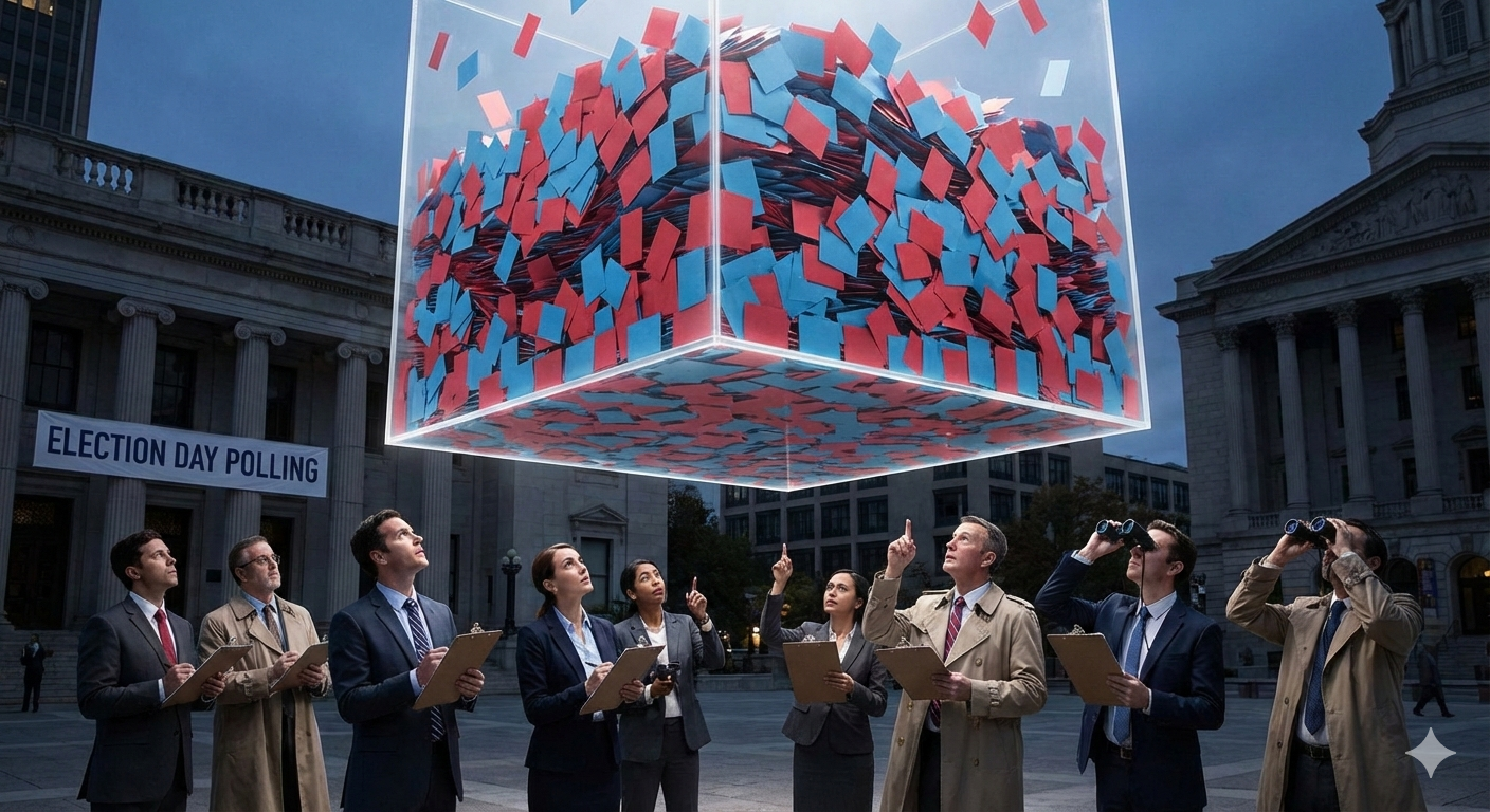
Imagine every state’s votes are publicly displayed in a giant transparent box suspended in midair, with red and blue slips.

Pollsters are standing on the ground, looking up, trying to guess the red and blue slip totals. Since it is impossible to count the millions of slips in the giant box, each pollster does their best to count slips in various parts (read: sample) of the box to get an estimate of the true count. They may each count different parts of the box and from different angles (read: different methodologies) and therefore their guesses will vary. The Central Limit Theorem¹ tells us that if you plot all these different estimates on a chart, they will cluster into a normal distribution (a bell curve) centered around the true vote counts.

Starting simple: Splitville

Consider a small state called Splitville with:

• 100 voters (not counting you)
• Two candidates: Alice and Bob
• Polls show a perfect 50–50 tie
• Polling error with a standard deviation (\(\sigma_D\)) of 5 votes

Let \(D\) denote the difference in votes between Alice and Bob. Since the polls show a tie, the expected difference is \(\mu_D = 0\). We can model the vote difference as a normal random variable:

A tie occurs when \(D=0\). To calculate the probability of this, we can apply a continuity correction and integrate the normal PDF over the interval \([-0.5, +0.5]\):

We can then use a midpoint Riemann approximation, since the PDF shouldn’t change much over this range. This yields:

This evaluates to 0.0797, or about an 8% chance of a tie in Splitville – pretty cool!

Revisiting the box analogy: national polling error

There is a big problem with our box analogy from earlier: what if there is a giant layer of red ballots sitting at the very top of every single box? Since every pollster is looking from below, none of them see those ballots. It doesn’t matter how many pollsters you have or how many “angles” they use – they are all going to miss those votes in the exact same way. This is systematic bias.

In practice, pollsters do their best to predict and correct for this, but this is why polling errors are highly correlated across states. In 2024, for example, the “hidden layer” favored Republicans, causing all seven swing states to move in the same direction.

To capture this effect, we need to decompose the polling error into two components ²:

• National error \(e_n\): The “hidden layer”. A shared shift that affects all states equally (e.g., polls systematically underestimating Republican turnout)
• State-specific error \(e_s\): The “different angles”. Independent noise for each state (e.g., local factors the polls missed)

The total polling error in a state is \(e_n + e_s\). We assume \(e_n \sim \mathcal{N}(0, \sigma_n^2)\) and \(e_s \sim \mathcal{N}(0, \sigma_s^2)\), where \(\sigma_n = 0.04\) and \(\sigma_s = 0.03\). Note that these are hyperparameters that seemed reasonable to me, not actually derived from historical data. Conveniently, since \(\sqrt{(0.03^2 + 0.04^2)} = 0.05\), our total error is 5%, matching historical error estimates.

The general formula

For any state, we define:

• \(N\) = number of voters
• \(m\) = polled margin as a fraction (e.g., a 55%–45% lead means \(m = 0.10\))
• \(e_n \sim \mathcal{N}(0, \sigma_n^2)\) = national polling error
• \(e_s \sim \mathcal{N}(0, \sigma_s^2)\) = state-specific polling error

Computing \(P(\text{vote flips state} \mid e_n)\)

We can factor a realized national error \(e_n\) into the margin itself, and then the vote difference follows:

A tie occurs when \(D = 0\), the probability of which is:

Simplifying:

Finally, we multiply by 0.5 to account for tiebreaker mechanics³:

Computing \(P(\text{vote flips election})\)

We want to compute:

We estimate these via Monte Carlo simulation:

where the expectation is over the national error \(e_n\) and the state errors for all other states.

Simulation Procedure

For each simulation:

1. Draw a national error: \(e_n \sim \mathcal{N}(0, \sigma_n^2)\)

2. For each state:

1. Compute the probability that a single vote flips the state outcome: $$ P(\text{vote flips state} \mid e_n) = \frac{0.5}{\sigma_s N \sqrt{2\pi}} \exp\!\left( -\frac{(m + e_n)^2}{2\sigma_s^2} \right) $$
2. For all other states, draw state-level errors: $$ e_s \sim \mathcal{N}(0, \sigma_s^2) $$
3. Compute realized margins for other states: $$ m + e_n + e_s $$
4. Check whether the state is pivotal (i.e., whether adding its electoral votes changes the election winner), and store the result as: $$ \mathbf{1}[\text{state flips election | vote flips state}] $$
5. Add the contribution to the running total: $$ P(\text{vote flips state} \mid e_n) \times \mathbf{1}[\text{state flips election | vote flips state}] $$

After all simulations, divide by the number of simulations to get:

Part 2: How much is the election actually worth?

Alright, we’ve figured out the probability side of the equation. Now for the hard part: what’s \(\Delta V\)? How much “value” does one candidate create over the other?

Before we dive in, note that everything we have calculated so far is independent of \(\Delta V\). The probability calculations remains the same regardless of what value you assign to the election. So while I am about to do a lot of hand-waving, it doesn’t actually matter: plug in your own \(\Delta V\); the analysis at the end holds too.

Also, \(\Delta V\) doesn’t have to be monetary. Feel free to measure it in lives saved, trees planted, vibes per capita, or whatever metric you care about. The framework is the same.

For the remainder of this post, I’ll use dollars as proxy for societal value.

The federal budget as a proxy

The 2024 federal budget was about $6.8T. Let’s break it down.

• ~$1T goes to paying interest (can’t really change that)
• ~$4T goes to mandatory spending (e.g. Social Security, Medicare – needs legislation to change)
• ~$1.8T is discretionary spending (this is what the president can actually influence)

Over a 4-year term, discretionary spending is about $7.2 trillion. But within this bucket, candidates don’t fully differ – both will still fund the military, run agencies, and pay for programs. So what we care about are the marginal differences.

Quantifying this marginal difference is difficult, and us voters should be pretty conservative here since policies can have second-order effects that are hard to predict ⁴. If our preferred candidate is 5% more effective with this money, that gives us $360B.

The president also influences via legislation, Supreme Court appointments, foreign policy, etc. which are hard to quantify. Let’s conveniently estimate the 4-year impact of all these other factors at $140B, giving us:

Putting it all together: 2024 election results

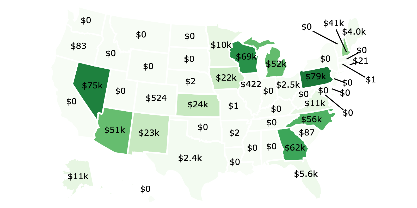
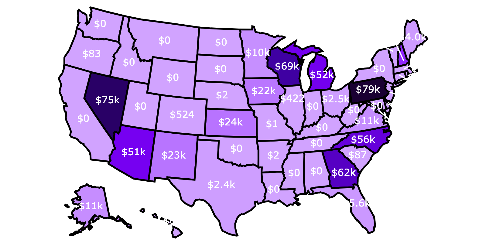
Let’s apply this framework to the 2024 presidential race. We used historical state-level polling margins and assumed a 4% national polling error and a 3% state specific polling error, set \(\Delta V\) to 500B, then ran 100 million simulations⁵. Here are the results (the table is scrollable):

What this actually means

The electoral college is absurd

The median U.S. voter has roughly a ~1 in 1 billion chance of swinging the election, whereas Pennsylvania voters have about a 1 in 6 million chance of swinging the election. In other words, the median U.S. voter is worth roughly ~0.5% of a Pennsylvanian.

What can I do in $NON_SWING_STATE?

If you live in a state where your EV is ~$0, not all hope is lost; there are a few ways you can still have agency:

Political activism

If you live in Oklahoma, your vote is worth ~43 cents. If you spend ten minutes on the phone convincing your cousin in Pennsylvania to vote, you have just performed a 180,000x force multiplier on your democratic power.

Vote swap

In the current U.S. equilibrium, due to the two party system, there are only two candidates ever “worth” voting for if you think in terms of expected value. That being said, there are still some people who vote for independent candidates, knowing damn well it is futile but presumably to “rage against the dying of the light”, as my friend put it.

This opens the door to vote swapping. If Dave the Democrat lives in a decided state (e.g. DC) and has a third-party friend Trent in a swing state (who prefers Democrat to Republican), they can arrange a swap: Trent votes Democrat and Dave votes third-party, both are happier. This is legal in the U.S., but requires trust to function.

Vote in local elections

In a local toss-up election with 10,000 voters, there is about a 1 in 125,000 chance of a tie – much more probable that your vote makes a difference. Moreover, since voter turnout is lower in local elections, political activism efforts become significantly more impactful.

Conclusion

This entire analysis is an elaborate cope for something I was probably going to do anyway. And it treats voting as a means to an end, a pure mathematical decision.

Of course, there are plenty of reasons to ignore the numbers and vote: self-expression, civic duty, or simply using Election Day as a forcing function to stay politically informed. All valid.

But now when someone claims my vote matters, or that the Electoral College is a good thing, I can whip out my probability density functions and simulations and end the conversation immediately. Not because I’ve won, but because literally no one cares.

◆ ◆ ◆

Thanks to draft readers Siddharth, Varun, Michael, and Madhav.